Truth, Damned Truth, and Statistics
Statistics may not be what floats your boat, but statistics can tell some important things about software development projects.
In this article, I'll show how even a very simple analysis of some basic project measurements can be exceedingly useful. The data in the following analysis is fake, but the situations they describe are from real projects.
A commercial software development project is a system that turns requirements into money. Therefore it makes sense to use economic measures, at least for a birds eye view of a project. If you have read my earlier postings, you will be familiar with the basic equation describing the state of a business system, the Return On Investment (ROI) equation:
ROI = (T - OE) / I
T = Throughput, the rate at which the project generates money. Because it is hard to put a monetary value on each unit of client valued functionality, this is commonly measured in Story Points, Function Points, or Feature Descriptions instead. I'll use Story Points, because it is the unit I am most comfortable with.
OE = Operating Expenses, the money expended by the project as it produces T. This includes all non-variable costs, including wages.
I = Inventory, money tied up in the system. This is the value of unfinished work, and assets that cannot be easily liquidated, like computers and software. Also called "Investment".
In this installment, I'll focus on Throughput, and a close relative, the Defect Rate. In a following article, I will discuss measuring Investment and Operating Expenses.
Throughput Diagram with Confidence Interval
Let's begin by looking at Throughput. The total Throughput of a project is the value added by the project. That is, if you get €300,000 for the project, then T = €300,000. A project is not an all or nothing deal. For example, the €300,000 project may have six partial deliveries. That would make each delivery worth €50,000. Normally, each partial delivery comprises several units of client valued functionality. A unit of client valued functionality is, for example, a use case. Thus, a use case represents monetary value.
Use cases do not make good units to measure Throughput, because they vary in size. Measuring Throughput in use cases would be like measuring ones fortune in bills, without caring about the denomination. However, a Story Point (SP), defined, for the purposes of this article, as the amount of functionality that can be implemented during one ideal working hour, has a consistent size. That is, a 40 SP use case is, on average, worth twice as much as a 20 SP use case. (This is of course a very rough approximation, but it is good enough for most development projects.)
We can estimate the size of use cases (or stories, if you prefer the XP term), in SP. Once we have done that, it is possible to measure Throughput. Just total the SPs of the use cases the team finishes in one iteration. The word "finished" means "tested and ready to deploy in a live application". No cheating!
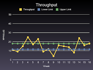
Figure 1: Throughput Per Week
Figure 1 shows the Throughput per week for a project over a 12 week period. As you can see, the productivity varies a lot. The diagram has two lines indicating the upper and lower control limits of the Throughput. Within the limits, or within the confidence interval, as it is also called, the project is in statistical control.
The control limits in this case are +- 3 standard deviations from the mean Throughput. What this means is that if the Throughput stays within the confidence interval each week, we have a stable production process, and we can, with 95% certainty, say that the future productivity will be within the limits set by the confidence interval.
If the Throughput is outside the control limits, as it is in Figure 1, the development process is out of control. This means that it is not possible to make predictions about the productivity of a week in the future based on past productivity. It also means it is useless for management to ask the developers how much work they can finish the next week.

Figure 2: Throughput Per Month
A project that is unpredictable in a short perspective, may well be predictable if you take a longer perspective. Figure 2 shows Throughput data for the same project, over the same time period as Figure 1. The difference is that the Throughput data has been aggregated into monthly figures. As you can see, the productivity for each month is pretty even, and well within the statistical control limits. The development team can, with 95% certainty, promise to deliver at least 47 SP each month. They can also promise an average production rate of 59 SP per month.
Given the Throughput, and the total number of SP for the project, it is possible to predict how long a project will take with fairly good accuracy. Obviously, such measurements must be continuously updated, because circumstances change. Requirements are added, or removed, the team may loose or add members, the code complexity tends to increase over time. All these factors, and many more, affect the Throughput over time, and may also cause a project to change from a controlled to an uncontrolled state.
Note that just because a project is in a controlled state, it does not mean the project is going well. A project that consistently has 0 Throughput is in a controlled state. Having the project in a controlled state does mean that we can make predictions about the future.
Having a project in a controlled state also means that if a project has problems, the causes are most likely to be systemic. That is, the problems arise from poor organization, a poor process, or outdated policy constraints, too little training, the wrong training, etc. Statistical Process Control (SPC) people call systemic causes "common causes".
Common cause problems must be fixed by the process owners, i.e. the management. The developers can't do much about it because the problem is out of their control.
When something happens that puts a project outside the predicted confidence interval, the cause is a random event. SPC people call random events "special causes". Special causes have to be dealt with on a case by case basis.
In practice, special causes are fairly rare. In the book Out Of the Crisis (1982), Edward Deming states that about 6% of all problems in production processes are due to special causes. The vast majority, 94%, of all problems have systemic causes. Much of the problems we experience in software projects are due to confusing special causes with common causes, i.e. causes of systemic failure.
A couple of years ago I worked in a project plagued with problems. Out of all the problems besetting the development team every day, only one problem was a special cause problem: we lost an afternoons work because we had to vacate the building. There was a fire in an adjacent building belonging to another company. The fire was a special cause of delay because it occurred only once. Had fires been a recurring problem, it would have been a common cause problem, and management would have had the responsibility to deal with it. (Three solutions off the top of my head: Get the other company evicted. Teach the other company safety procedures so there are no more fires. Move to other, safer, premises.)
Let's focus on common causes. They are the most interesting, because the vast majority of problems fall in this category. The problem with common causes are that management usually fails to identify them for what they are. the failure to identify common causes is of course itself a systemic failure, and has a common cause. (I leave it to you to figure out what it is. It should not be too hard.) The result is that management resorts to firefighting techniques, which leaves the root cause unaffected. Thus, it won't be long until the problem crops up again.
The first thing to do with a problem is to notice that it is there. The second thing to do is to put it in the right category. A diagram with a confidence interval can help you do both.
Once you know the problem is there, you can track it down using some form of root cause analysis, for example Five Why, or a Current Reality Tree (from the TOC Thinking Tools). My advice is to start with Five Why, because it is a very simple method, and then switch to the TOC Thinking Tools if the problem proves hard to identify, you suspect many causes, or if it is not immediately obvious how to deal with the problem.
Defect Diagram With Confidence Interval
The Throughput diagram does not give a complete picture of how productive a project is. It is quite common for a development team to produce new functionality very quickly, but with poor quality. This means a lot of the development effort can be spent on rework. I won't go into the economic details in this article, but fixing defects may account for a substantial part of the cost of a project. In addition, defects cause customers to be dissatisfied, which can cause even greater losses. A high defect rate is also an indicator of a high level of complexity in the code. This complexity reduces Throughput, and in most cases it is not necessary. (I haven't seen a commercial mid to large software development project yet that did not spend a lot of effort dealing with complexity that did not have to be there in the first place.)

Figure 3: Defect Graph
Figure 3 shows a defect graph. These are defects caught by a test team doing inspection type testing, or by customers doing acceptance testing, or using the code. It is important to note that the graph shows when defects were created, not when they were detected. This is important to know, because if you do not know when defects where created, you won't know if process improvements you make have any effect on the defect rate. If you measure when defects are detected, as most projects do, there may be years until you see any effects from an improved process.
In this case, the defect rate is within the control limits all the time, which means the defects that do occur are a systemic problem. The control limits are rather far apart, indicating a process with a lot of variation in results. Reducing the defect rate is clearly a management problem.
The Limitations of Calculating the Confidence Interval
The confidence interval method has several limitations. First of all, you need a process that varies within limits. If you measure something that has a continuous increasing or declining trend, confidence intervals won't be very useful.
Second, the method can detect only large shifts, on the order of 1.5 standard deviations or more. For example, in Figure 3, the number of defects seem to be declining, but all data points are within the confidence interval. It is impossible to say whether the number of defects are really going down, or if there are just two lucky months in a row. Thus, if some method of defect prevention was instigated at the beginning of month 2, it is not possible to tell if these measures had any real effect. A more sophisticated statistical method, like Exponentially Weighted Moving Average (EWMA), could probably have determined this.
Third, it is assumed that the data points are relatively independent of each other. This is likely to be the case in a well run project, but in a badly organized project, the Throughput may be influenced by a wave phenomenon caused by excessive Inventory. (I'll discuss that in the next article in this series.) When such conditions exist, the confidence interval looses its meaning. On the up side, excessive Inventory shows up very clearly in a Design In Process graph, so management can still get on top of the problem.
Calculating a confidence interval for a chart is still useful in many cases. It is a simple method. Any statistical package worth its salt has support for it. (I used the Statarray Ruby package, and drew the graphs with Gruff. You can find it on RubyForge.)


Comments